Using data from pysat (with EAB)
This example showcases Equatorward Auroral Boundaries (EABs), while
demonstrating how to use pysat with ocbpy.
Using Equatorward Auroral Boundaries
EABs may be loaded using the EABoundary class.
This is a wrapper for the OCBoundary class with
different defaults more appropriate for EABs. Currently,
IMAGE and DMSP SSJ both have EAB data. This
example uses the default file for IMAGE from the Northern hemisphere. It is
very similar to Getting Started, the first example in this section.
import ocbpy

eab = ocbpy.EABoundary(instrument='image', hemisphere=1)
print(eab)

EABoundary file: ~/ocbpy/ocbpy/boundaries/image_north_circle.eab
Source instrument: IMAGE
Boundary reference latitude: 64.0 degrees

305861 records from 2000-05-03 02:41:43 to 2002-10-31 20:05:16

YYYY-MM-DD HH:MM:SS Phi_Centre R_Centre R
------------------------------------------
2000-05-03 02:41:43 251.57 5.45 14.16
2000-05-05 11:35:27 111.80 2.34 25.12
...
2002-10-31 20:03:16 354.41 6.22 20.87
2002-10-31 20:05:16 2.87 14.67 13.10

Uses scaling function(s):
ocbpy.ocb_correction.circular(**{})
To prepare to use the EAB data, find the time with the first quality boundary.
The expected record index, eab.rec_ind, is 1.
eab.get_next_good_ocb_ind()
Load a pysat Instrument (Madrigal TEC)
Total Electron Content (TEC) is one of the most valuable ionospheric data sets.
Madrigal provides Vertical TEC (VTEC) maps
from the 1990’s onward that specify the median VTEC in 1 degree x 1 degree
geographic latitude x longitude bins. The
pysat package,
pysatMadrigal
has an instrument for obtaining, managing, and processing this VTEC data. To
run this example, you must have pysatMadrigal
installed.
After setting up pysat, download the file needed for this example
using the following commands.
import pysat
import pysatMadrigal as py_mad

# Replace `user` with a string holding your name and `password` with your
# email.  Madrigal uses these to demonstrate their utility to funders.
tec = pysat.Instrument(inst_module=py_mad.instruments.gnss_tec, tag='vtec',
                       user=user, password=password)
tec.download(start=eab.dtime[eab.rec_ind])
print(tec.files.files)

2000-05-04    gps000504g.001.netCDF4
2000-05-05    gps000505g.001.netCDF4
2000-05-06    gps000506g.001.netCDF4
dtype: object
pysat makes it possible to perform well-defined data analysis
prodedures while loading the desired data. The
ocbpy.instrument.pysat_instrument module contains functions that may
be applied using the pysat custom interface. The
EAB conversion can handle magnetic, geodetic, or geocentric coordinates for
scalar or vector data types using the loc_coord and
vect_coord keyword arguments, respectively. We do need to calculate
local time before calculating the EAB coordinates, though.
def add_slt(inst, lon='glon', slt='slt'):
    """Add solar local time.

    Parameters
    ----------
    inst : pysat.Instrument
        Data object
    lon : str
        Geographic longitude key (default='glon')
    slt : str
        Key for new solar local tim data (default='slt')

    """
    # Initalize the data arrays
    lt = [ocbpy.ocb_time.glon2slt(inst[lon], dtime) for dtime in inst.index]

    # Assign the SLT data to the input Instrument
    inst.data = inst.data.assign({slt: (("time", lon), lt)})
    return
Assign this function and the ocbpy function in the desired order of
operations. When calculating magnetic coordinates, it is important to specify
the height, which can be a single value or specified for each observation.
tec.custom_attach(add_slt, kwargs={'lon': 'glon'})
tec.custom_attach(ocbpy.instruments.pysat_instruments.add_ocb_to_data,
                  kwargs={'ocb': eab, 'mlat_name': 'gdlat',
                  'mlt_name': 'slt', 'height_name': 'gdalt',
                  'loc_coord': 'geodetic', 'max_sdiff': 150})
tec.load(date=eab.dtime[eab.rec_ind])
print(tec.variables)

['time', 'gdlat', 'glon', 'dtec', 'gdalt', 'tec', 'gdlat_eab',
 'slt_eab', 'r_corr_eab']
Now we have the EAB coordinates for each location in the Northern Hemisphere where a good EAB was found within 2.5 minutes of the data record. This time difference was chosen because the VTEC data has a 5 minute resolution.
Now, let’s plot the average of the VTEC equatorward of the EAB. To do this we will first need to calculate these averages.
del_lat = 2.0
del_mlt = 2.0
ave_lat = np.arange(45, eab.boundary_lat, del_lat)
ave_mlt = np.arange(0, 24, del_mlt)
ave_tec = np.full(shape=tec['tec'].shape, fill_value=np.nan)

for lat in ave_lat:
    for mlt in ave_mlt:
        # We are not overlapping bins, so don't need to worry about MLT
        # rollover from 0-24
        sel_tec = tec['tec'].where(
            (tec['gdlat_eab'] > lat) & (tec['gdlat_eab'] <= lat + del_lat)
            & (tec['slt_eab'] >= mlt) & (tec['slt_eab'] < mlt + del_mlt))
        inds = np.where(~np.isnan(sel_tec.values))
        if len(inds[0]) > 0:
            ave_tec[inds] = np.nanmean(sel_tec.values)
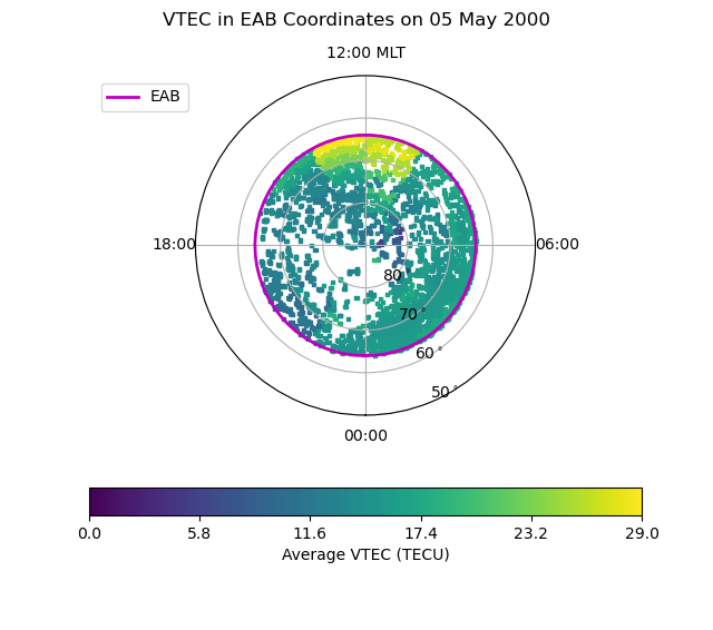
Now let us plot these averages at the EAB location of each measurement. This will provide us with knowledge of the coverage as well as knowledge of the average behaviour of the sub-auroral VTEC on this day.
# Initialise the figure
fig = plt.figure()
fig.suptitle("VTEC in EAB Coordinates on {:}".format(
    tec.date.strftime('%d %B %Y')))
ax = fig.add_subplot(111, projection="polar")
ax.set_theta_zero_location("S")
ax.xaxis.set_ticks([0, 0.5 * np.pi, np.pi, 1.5 * np.pi])
ax.xaxis.set_ticklabels(["00:00", "06:00", "12:00 MLT", "18:00"])
ax.set_rlim(0, 40)
ax.set_rticks([10, 20, 30, 40])
ax.yaxis.set_ticklabels(["80$^\circ$", "70$^\circ$", "60$^\circ$",
                         "50$^\circ$"])

# Add the boundary location
lon = np.arange(0.0, 2.0 * np.pi + 0.1, 0.1)
lat = np.ones(shape=lon.shape) * (90.0 - eab.boundary_lat)
ax.plot(lon, lat, "m-", linewidth=2, label="EAB")

# Plot the VTEC data
tec_lon = (tec['slt_eab'].values * np.pi / 12.0)
tec_lat = (90.0 - tec['gdlat_eab'].values)
tec_max = np.ceil(np.nanmax(ave_tec))
con = ax.scatter(tec_lon, tec_lat, c=ave_tec.transpose([0, 2, 1]),
                 marker="s", cmap=mpl.colormaps["viridis"], s=5,
                 vmin=0, vmax=tec_max)

# Add a colourbar and labels
tticks = np.linspace(0, tec_max, 6, endpoint=True)
cb = fig.colorbar(ax.collections[0], ax=ax, ticks=tticks,
                  orientation='horizontal')
cb.set_label('Average VTEC (TECU)')
ax.legend(fontsize='medium', bbox_to_anchor=(0.0, 1.0))