DMSP SSJ Boundaries
For more information about these boundaries, see Section DMSP SSJ.
Loading DMSP SSJ Boundaries
Unlike the IMAGE and AMPERE boundaries, the DMSP SSJ boundaries are not included
with the package. However, routines to obtain them are. To use them, you used to
need the
ssj_auroral_boundary
package, but now we preferentially support using the
zendodo_get package to obtain the
boundary files from their archive at the website: zenodo.org/record/3373812.
Once installed, you can download DMSP SSJ data and obtain a boundary file for a
specified time period (or all available times) using
ocbpy.boundaries.dmsp_ssj_files. For this example, we’ll use a single
day. You can download the files into any directory, but this example will put
them in the same directory as the other boundary files.
import datetime as dt
import matplotlib.pyplot as plt
import ocbpy
import os

stime = dt.datetime(2010, 12, 31)
etime = stime + dt.timedelta(days=1)
out_dir = os.path.join(os.path.split(ocbpy.__file__)[0], "boundaries")

# Set `use_dep=True` in the function below to use the deprecated subroutines
bfiles = ocbpy.boundaries.dmsp_ssj_files.fetch_format_ssj_boundary_files(
    stime, etime, out_dir=out_dir, rm_temp=False)
By setting rm_temp=False, all of the different DMSP files will be kept in
the specified output directory. If you set use_dep=True you should have
three CDF files (the data downloaded from each DMSP spacecraft), the CSV files
(the boundaries calculated for each DMSP spacecraft) and four boundary files.
Otherwise you will have a zip archive, the CSV files, and the boundary files.
The boundary files have an extention of .eab for the Equatorial Auroral
Boundary and .ocb for the Open-Closed field line Boundary. The files are
separated by hemisphere, and also specify the date range. Because only one day
was obtained, the start and end dates in the filename are identical. When
rm_temp=True, the zip archive (or CDF files) and CSV files are removed.
You can now load the DMSP SSJ boundaries by specifying the desired filename, instrument, and hemisphere or merely the instrument and hemisphere.
# Load with filename, instrument, and hemisphere
south_file = os.path.join(out_dir,
                          "dmsp-ssj_south_20101231_20101231_v1.1.2.ocb")
ocb_south = ocbpy.OCBoundary(filename=south_file, instrument='dmsp-ssj',
                             hemisphere=-1)
print(ocb_south)

OCBoundary file: ~/ocbpy/ocbpy/boundaries/dmsp-ssj_south_20101231_20101231_v1.1.2.ocb
Source instrument: DMSP-SSJ
Boundary reference latitude: -74.0 degrees

21 records from 2010-12-31 00:27:23 to 2010-12-31 22:11:38

YYYY-MM-DD HH:MM:SS Phi_Centre R_Centre R
-----------------------------------------------------------------------------
2010-12-31 00:27:23 356.72 14.02 12.13
2010-12-31 12:27:56 324.82 0.86 14.73
...
2010-12-31 18:49:58 233.68 6.12 14.10
2010-12-31 22:11:38 318.60 4.64 12.34

Uses scaling function(s):
ocbpy.ocb_correction.circular(**{})

# Load with date, instrument, and hemisphere
ocb_north = ocbpy.OCBoundary(stime=stime, instrument='dmsp-ssj',
                             hemisphere=1)
print(ocb_north)

OCBoundary file: ~/ocbpy/ocbpy/boundaries/dmsp-ssj_north_20101231_20101231_v1.1.2.ocb
Source instrument: DMSP-SSJ
Boundary reference latitude: 74.0 degrees

27 records from 2010-12-31 01:19:13 to 2010-12-31 23:02:48

YYYY-MM-DD HH:MM:SS Phi_Centre R_Centre R
-----------------------------------------------------------------------------
2010-12-31 01:19:13 191.07 10.69 8.59
2010-12-31 06:27:18 195.29 13.52 6.77
...
2010-12-31 21:21:32 259.27 2.73 10.45
2010-12-31 23:02:48 234.73 3.94 10.79

Uses scaling function(s):
ocbpy.ocb_correction.circular(**{})
The circular scaling function with no input adds zero the the boundaries, and so performs no scaling.
Using DMSP SSJ Boundaries
Because DMSP SSJ Boundaries are only measured along a satellite track, you
cannot use these boundaries to convert between magnetic and OCB or Dual-boundary
coordinates at just any location or local time. To address this issue, the
ocbpy.cycle_boundary.satellite_track() function can be used to
determine whether or not a location is close enough to the satellite track.
This example shows the width along the linear approximation of the satellite
track allowed along the Boundary latitude. The axis formatting is performed
using the set_up_polar_plot function defined in the
Coordinate Convertion example.
# Set up the figure
fig = plt.figure()
ax = fig.add_subplot(111, projection="polar"
set_up_polar_plot(ax, hemi=ocb_south.hemisphere)

# Get the OCB location in AACGM coordinates
mlt = np.linspace(0, 24, 64)
ocb_south.get_aacgm_boundary_lat(mlt)

# Plot the OCB location
ax.plot(mlt * np.pi / 12.0,
        90 + ocb_south.aacgm_boundary_lat[ocb_south.rec_ind], "m-", lw=2,
        label="OCB")

# Deterimine which OCB locations are along the satellite track
igood = ocbpy.cycle_boundary.satellite_track(
    ocb_south.aacgm_boundary_lat[ocb_south.rec_ind],
    ocb_south.aacgm_boundary_mlt[ocb_south.rec_ind],
    ocb_south.x_1[ocb_south.rec_ind], ocb_south.y_1[ocb_south.rec_ind],
    ocb_south.x_2[ocb_south.rec_ind], ocb_south.y_2[ocb_south.rec_ind],
    hemisphere=ocb_south.hemisphere)
ax.plot(mlt[igood] * np.pi / 12.0,
        90 + ocb_south.aacgm_boundary_lat[ocb_south.rec_ind][igood], "ks",
        label="Measured OCB")
The default constraints for ocbpy.cycle_boundary.satellite_track()
allow a 1 degree deviation in either Cartesian direction and a maximum distance
of 5 degrees equatorward of the Boundary.
lat = np.arange(-90, -60, 1)
grid_mlt, grid_lat = np.meshgrid(mlt, lat)
grid_mlt = grid_mlt.flatten()
grid_lat = grid_lat.flatten()

igood = ocbpy.cycle_boundary.satellite_track(
    grid_lat, grid_mlt, ocb_south.x_1[ocb_south.rec_ind],
    ocb_south.y_1[ocb_south.rec_ind], ocb_south.x_2[ocb_south.rec_ind],
    ocb_south.y_2[ocb_south.rec_ind], hemisphere=ocb_south.hemisphere)
ax.plot(grid_mlt[~igood] * np.pi / 12.0, 90 + grid_lat[~igood], ".",
        color="palegreen", label="Data", zorder=1)
ax.plot(grid_mlt[igood] * np.pi / 12.0, 90 + grid_lat[igood], "g.",
        label="Satellite track data")
ax.legend(loc=2, title="{:}".format(ocb_south.dtime[ocb_south.rec_ind]),
          bbox_to_anchor=(-0.4, 1.15))
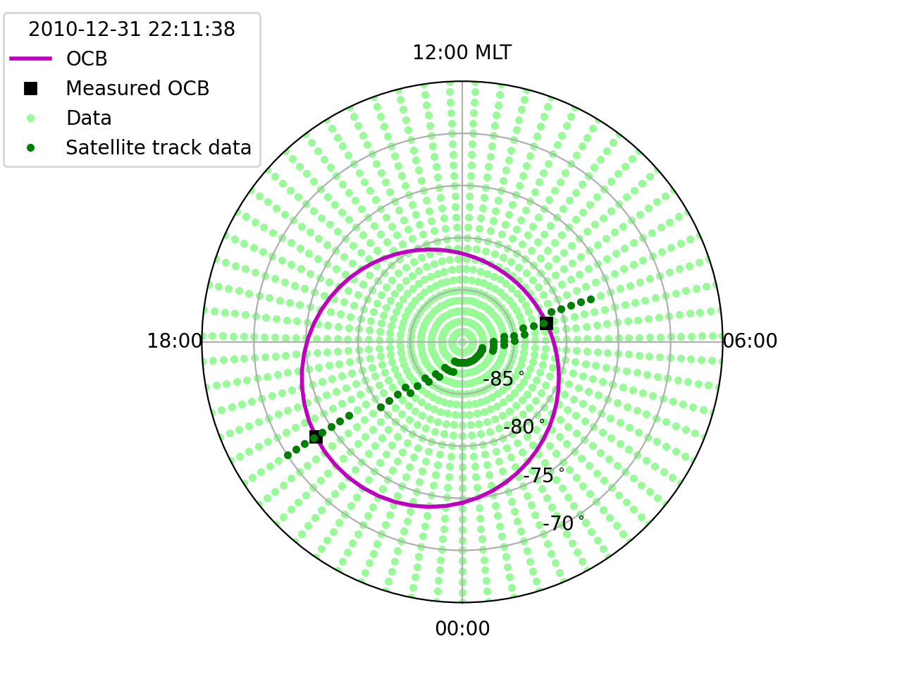
Note that because the OCB is determined based off of only two points, the OCB MLT is not very accurate. With poorly defined OCBs, we recommend using only the gridded latitude along the satellite track.