Using Model Boundaries
The boundary models supplied in this package can be used in various ways. The boundary locations themselves can be calculated for a range of MLTs and upstream conditions and extracted for various uses. They can also be used to grid data in adaptive coordinates, as if they were a boundary data set. This may be useful for statistical studies where sufficient observations of the desired boundaries are not available.
Calculate Boundary Locations
Following on from the model OCBoundary initialisation example
(see Initialising with a Model), the OCB locations for the desired period of time can
be calculated for a set of MLTs using the
get_aacgm_boundary_lat() method.
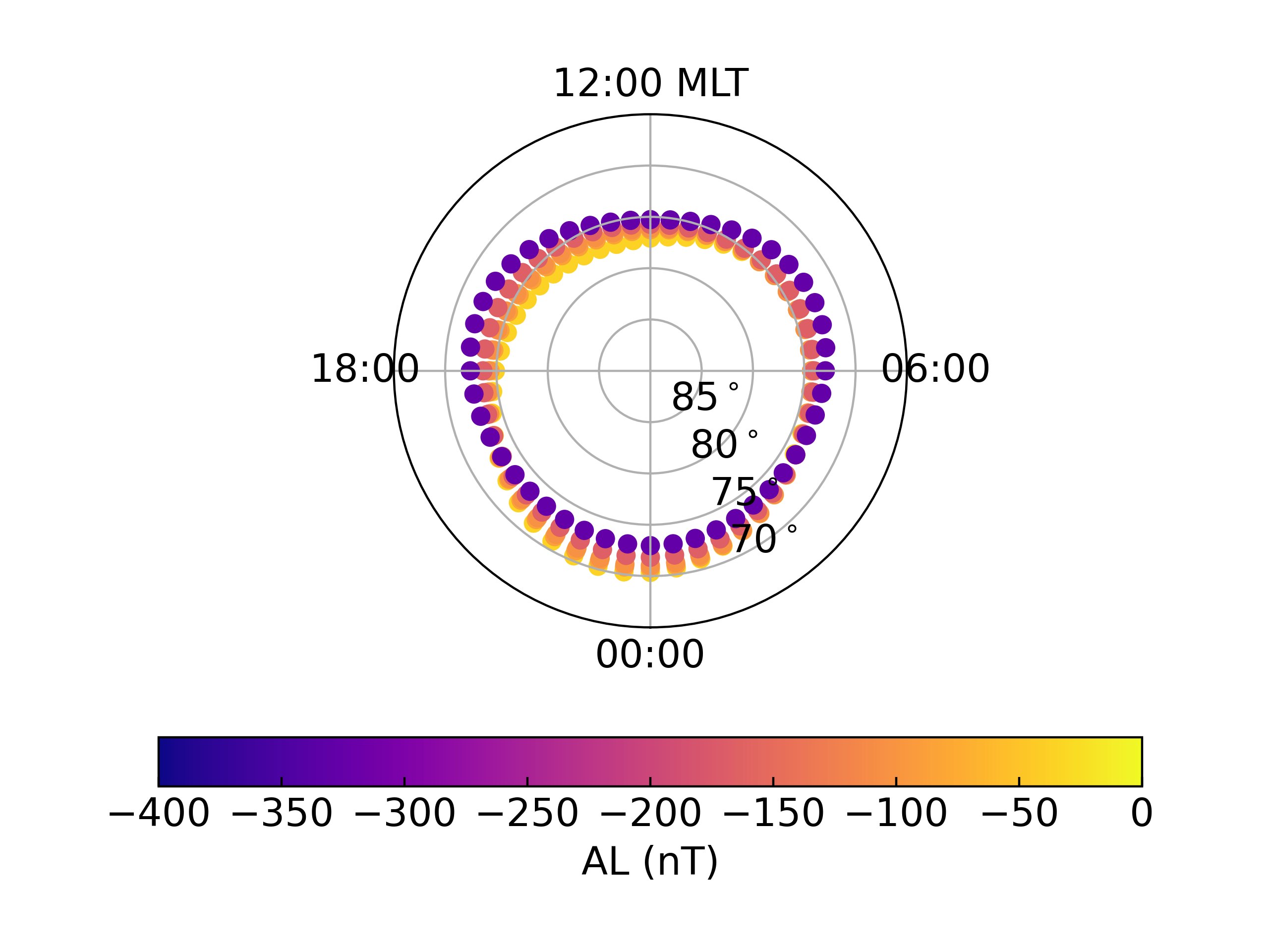
import numpy as np

# Define the desired MLT range
mlt = np.arange(0, 24, 0.5)

# Calculate the boundaries at all times
starkov.get_aacgm_boundary_lat(mlt)
This provides the AACGMV2 magnetic latitude for the entire range of MLT at the specified AL values. We can plot these boundaries, using the formatting function previously defined in set_up_polar_plot.
# Set up fthe figure
fig = plt.figure()
ax = fig.add_subplot(111, projection='polar')
set_up_polar_plot(ax)

# Construct an array of AL values to color code the boundaries
al_array = np.full(shape=(mlt.shape[0], starkov.records),
                   fill_value=al_list).transpose()

# Plot the boundaries
con = ax.scatter(np.asarray(starkov.aacgm_boundary_mlt) * np.pi / 12.0,
                 90 - np.asarray(starkov.aacgm_boundary_lat), c=al_array,
                 marker='.', vmin=-400, vmax=0,
                 cmap=mpl.colormaps.get_cmap('plasma'))

# Add a colorbar
cb = fig.colorbar(con, ax=ax, orientation='horizontal')
cb.set_label('AL (nT)')
Calculate Boundary Locations
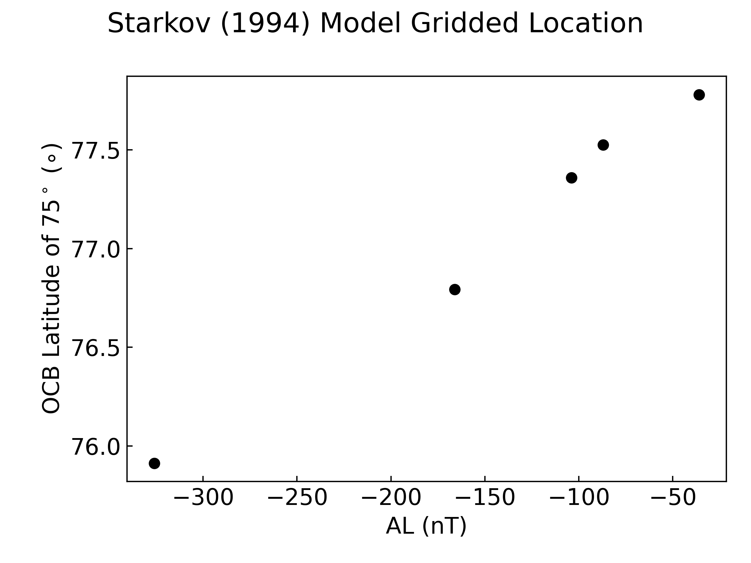
You can also use these empirical boundaries to grid data. When using models to do this, be aware that the accuracy of the model will impact the results of any statistical studies. The example below tracks the location of a location near the edge of the polar cap at magnetic midnight.
# Ensure the record index iterator is at zero to start
starkov.rec_ind = 0

# Cycle through each time and find the OCB location of the magnetic pole
ocb_lat = list()
ocb_mlt = list()
while starkov.rec_ind < starkov.records:
    out = starkov.normal_coord(75.0, 0.0, height=0.0)
    ocb_lat.append(out[0])
    ocb_mlt.append(float(out[1]))
    starkov.rec_ind += 1

# Note that this model is consistently centred at the same location, so
# MLT does not change
print(ocb_mlt)  # Will show all 0.0

# Plot the change in OCB latitude as a function of AL
fig = plt.figure()
ax = fig.add_subplot(111)
ax.plot([rkwargs['al'] for rkwargs in starkov.rfunc_kwargs], ocb_lat, 'ko')

# Format the figure
ax.set_xlabel('AL (nT)')
ax.set_ylabel('OCB Latitude of 75$^\circ$ ($\circ$)')
fig.suptitle("Starkov (1994) Model Gridded Location")
fig.tight_layout()