Load a general data file (DMSP SSIES)
DMSP SSIES provides commonly used polar data, which can be accessed from Madrigal, which also has a Python API called madrigalWeb. To run this example, follow the previous link(s) and download the ASCII file for F15 on 23 May 2000. Choosing the UT DMSP with quality flags for the best calcuations of ion drift and selecting ASCII instead of HDF5 will provide you with a file named dms_ut_20000523_15.002.txt. To load this file, use the following commands.
import datetime as dt
import numpy as np
import matplotlib as mlt
import matplotlib.pyplot as plt
import ocbpy

hh = ["YEAR     MONTH      DAY       HOUR      MIN       SEC       RECNO     KINDAT      KINST       UT1_UNIX        UT2_UNIX       GDALT      GDLAT      GLON       MLAT         MLT      ION_V_SAT_FOR ION_V_SAT_LEFT VERT_ION_V       NI           PO+           PHE+         PH+        TI         TE     RPA_FLAG_UT IDM_FLAG_UT     RMS_X        SIGMA_VY      SIGMA_VZ"]
dmsp_filename = "dms_ut_20000423_15.002.txt"
dmsp_head, dmsp_data = ocbpy.instruments.general.load_ascii_data(dmsp_filename, 1, datetime_cols=[0, 1, 2, 3, 4, 5], header=hh, datetime_fmt="%Y %m %d %H %M %S", int_cols=[6, 7, 8, 25, 26])

print(dmsp_data['TI'].shape, dmsp_data.keys())

(200060,), ['PH+', 'KINST', 'MIN', 'RPA_FLAG_UT', 'KINDAT', 'datetime', 'MLAT', 'UT2_UNIX', 'ION_V_SAT_FOR', 'ION_V_SAT_LEFT', 'GDALT', 'UT1_UNIX', 'GDLAT', 'HOUR', 'PHE+', 'IDM_FLAG_UT', 'SIGMA_VZ', 'SIGMA_VY', 'SEC', 'RMS_X', 'TI', 'TE', 'DAY', 'GLON', 'NI', 'RECNO', 'PO+', 'MLT', 'YEAR', 'MONTH', 'VERT_ION_V']
In the call to ocbpy.instruments.general.load_ascii_data(), quality
flags and number of points are saved as integers by specifying int_cols. The
header may not need to be specified using header; have a go loading
it without this keyword arguement. The results will be the same as long as
there are no errors in the file header specification.
Before calculating the OCB coordinates, add space in the data dictionary for the OCB coordinates and find out which data have a good quality flag.
ram_key = 'ION_V_SAT_FOR'
rpa_key = 'RPA_FLAG_UT'
idm_key = 'IDM_FLAG_UT'
dmsp_data['OCB_MLT'] = np.full(shape=dmsp_data[ram_key].shape,
                               fill_value=np.nan)
dmsp_data['OCB_LAT'] = np.full(shape=dmsp_data[ram_key].shape,
                               fill_value=np.nan)
igood = np.where((dmsp_data[rpa_key] < 3) & (dmsp_data[idm_key] < 3))
print(len(igood[0]), dmsp_data[ram_key][igood].max(),
      dmsp_data[ram_key][igood].min())

7623 978.0 -2159.0
Now get the OCB coordinates for each location. This will not be possible everywhere, since IMAGE doesn’t provide Southern Hemisphere data and only times with a good OCB established within the last 5 minutes will be used.
idmsp = 0
ndmsp = len(igood[0])
ocb = ocbpy.OCBoundary()
ocb.get_next_good_ocb_ind()

print(idmsp, ndmsp, ocb.rec_ind, ocb.records)

0 7623 0 305805
This is the starting point for cycling through the records.
while idmsp < ndmsp and ocb.rec_ind < ocb.records:
    idmsp = ocbpy.match_data_ocb(ocb, dmsp_data['datetime'][igood],
                                 idat=idmsp, max_tol=600)
    if idmsp < ndmsp and ocb.rec_ind < ocb.records:
        nlat, nmlt, r_corr = ocb.normal_coord(
            dmsp_data['MLAT'][igood[0][idmsp]],
            dmsp_data['MLT'][igood[0][idmsp]])
        dmsp_data['OCB_LAT'][igood[0][idmsp]] = nlat
        dmsp_data['OCB_MLT'][igood[0][idmsp]] = nmlt
        idmsp += 1

igood = np.where(~np.isnan(dmsp_data['OCB_LAT']))
print(len(igood[0]), dmsp_data['OCB_LAT'][igood].max())

2218 89.5098551674689
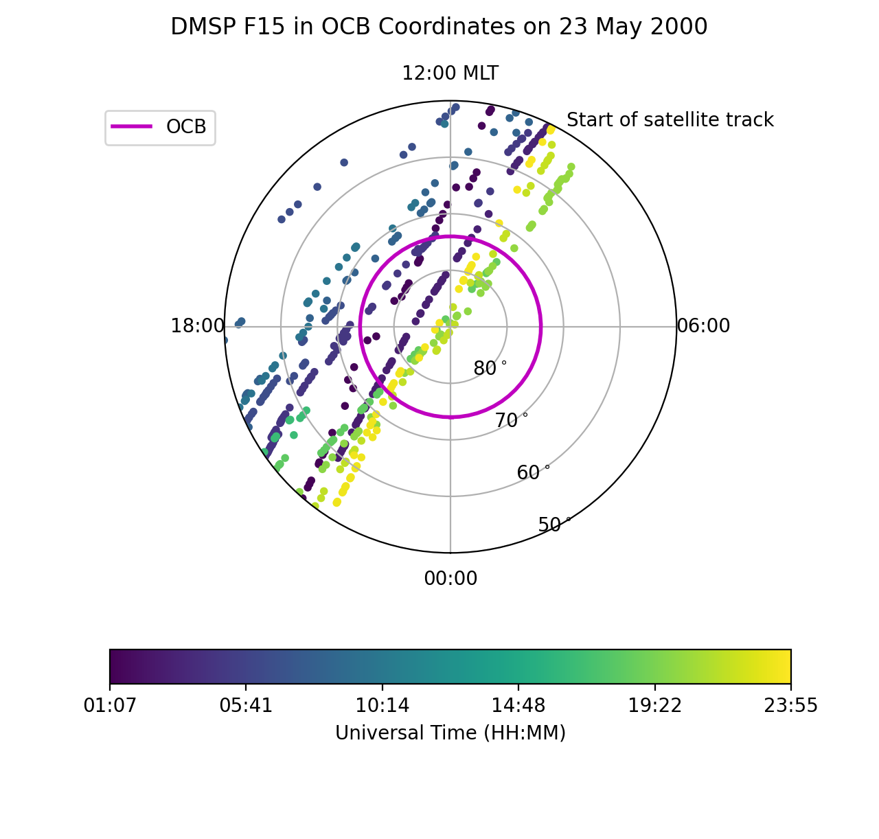
Now, let’s plot the satellite track over the pole, relative to the OCB, with the location accouting for changes in the OCB at a 5 minute resolution. Note how the resolution results in apparent jumps in the satellite location. We aren’t going to plot the ion velocity here, because it is provided in spacecraft coordinates rather than magnetic coordinates, adding an additional (and not intensive) level of processing.
fig = plt.figure()
fig.suptitle("DMSP F15 in OCB Coordinates on {:}".format(
    dmsp_data['datetime'][igood][0].strftime('%d %B %Y')))
ax = fig.add_subplot(111, projection="polar")
ax.set_theta_zero_location("S")
ax.xaxis.set_ticks([0, 0.5 * np.pi, np.pi, 1.5 * np.pi])
ax.xaxis.set_ticklabels(["00:00", "06:00", "12:00 MLT", "18:00"])
ax.set_rlim(0, 40)
ax.set_rticks([10, 20, 30, 40])
ax.yaxis.set_ticklabels(["80$^\circ$", "70$^\circ$", "60$^\circ$",
                         "50$^\circ$"])

lon = np.arange(0.0, 2.0 * np.pi + 0.1, 0.1)
lat = np.ones(shape=lon.shape) * (90.0 - ocb.boundary_lat)
ax.plot(lon, lat, "m-", linewidth=2, label="OCB")

dmsp_lon = dmsp_data['OCB_MLT'][igood] * np.pi / 12.0
dmsp_lat = 90.0 - dmsp_data['OCB_LAT'][igood]
dmsp_time = mpl.dates.date2num(dmsp_data['datetime'][igood])
ax.scatter(dmsp_lon, dmsp_lat, c=dmsp_time, cmap=mpl.cm.get_cmap("viridis"),
           marker="o", s=10)
ax.text(10 * np.pi / 12.0, 41, "Start of satellite track")

tticks = np.linspace(dmsp_time.min(), dmsp_time.max(), 6, endpoint=True)
dticks = ["{:s}".format(mpl.dates.num2date(tval).strftime("%H:%M"))
          for tval in tticks]
cb = fig.colorbar(ax.collections[0], ax=ax, ticks=tticks,
                  orientation='horizontal')
cb.ax.set_xticklabels(dticks)
cb.set_label('Universal Time (HH:MM)')
ax.legend(fontsize='medium', bbox_to_anchor=(0.0,1.0))