Coordinate Convertion

All Boundary classes have methods to convert between magnetic, geodetic, or geographic and normalised boundary coordinates. When geodetic or geographic coordinates are provided, aacgmv2 is used to perform the conversion at a specified height.

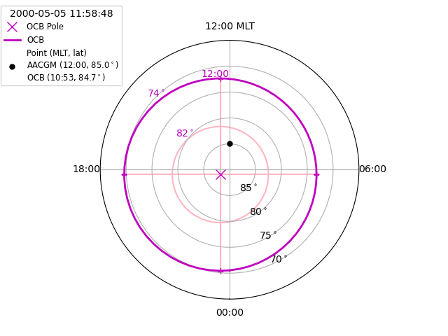
Convert between AACGM and OCB coordinates

We’ll start by visualising the location of the OCB using the first good OCB in the default IMAGE FUV file.

def set_up_polar_plot(ax, hemi=1):
    """Set the formatting for a polar plot.

    Parameters
    ----------
    ax : Axes object
        Subplot Axes object to be formatted
    hemi : int
        Hemisphere, 1 is North and -1 is South (default=1)

    """
    ss = "" if hemi == 1 else "-"
    ax.set_theta_zero_location("S")
    ax.xaxis.set_ticks([0, 0.5 * np.pi, np.pi, 1.5 * np.pi])
    ax.xaxis.set_ticklabels(["00:00", "06:00", "12:00 MLT", "18:00"])
    ax.set_rlim(0, 25)
    ax.set_rticks([5, 10, 15, 20])
    ax.yaxis.set_ticklabels([ss + "85$^\circ$", ss + "80$^\circ$",
                             ss + "75$^\circ$", ss + "70$^\circ$"])
    return

fig = plt.figure()
ax = fig.add_subplot(111, projection="polar")
set_up_polar_plot(ax)

Mark the location of the circle centre in AACGM coordinates

# Use the OCB of the first good, paired OCB loaded in the `dual` example
ocb.rec_ind = dual.ocb_ind[0]
ax.plot(np.radians(ocb.phi_cent[ocb.rec_ind]), ocb.r_cent[ocb.rec_ind],
        "mx", ms=10, label="OCB Pole")

Calculate and plot the location of the OCB in AACGM coordinates

mlt = np.linspace(0.0, 24.0, num=64)
ocb.get_aacgm_boundary_lat(mlt, rec_ind=ocb.rec_ind)
theta = ocbpy.ocb_time.hr2rad(mlt)
rad = 90.0 - ocb.aacgm_boundary_lat[ocb.rec_ind]
ax.plot(theta, rad, "m-", linewidth=2, label="OCB")
ax.text(theta[40], rad[40] + 2, "{:.0f}$^\circ$".format(ocb.boundary_lat),
        fontsize="medium", color="m")

Add more reference labels for OCB coordinates. Since we know the location that we want to place these labels in OCB coordinates, the revert_coord() method can be used to get the location in AACGM coordinates.

# Define a latitude grid for the OCB coordinates
grid_ocb = 0.5 * (90 - abs(ocb.boundary_lat)) + ocb.boundary_lat
grid_lat, grid_mlt = ocb.revert_coord(grid_ocb, mlt)
grid_lat = 90.0 - grid_lat
grid_theta = grid_mlt * np.pi / 12.0

# Define the MLT grid in OCB coordinates
lon_clock = list()
lat_clock = list()
for ocb_mlt in np.arange(0.0, 24.0, 6.0):
    aa, oo = ocb.revert_coord(ocb.boundary_lat, ocb_mlt)
    lon_clock.append(oo * np.pi / 12.0)
    lat_clock.append(90.0 - aa)

# Plot the OCB latitude and MLT grid
ax.plot(lon_clock, lat_clock, "m+")
ax.plot([lon_clock[0], lon_clock[2]], [lat_clock[0], lat_clock[2]], "-",
        color="lightpink", zorder=1)
ax.plot([lon_clock[1], lon_clock[3]], [lat_clock[1], lat_clock[3]], "-",
        color="lightpink", zorder=1)
ax.plot(grid_theta, grid_lat, "-", color="lightpink", zorder=1)
ax.text(lon_clock[2] + .2, lat_clock[2] + 1.0, "12:00",fontsize="medium",
        color="m")
ax.text(grid_theta[40], grid_lat[40] + 2, "{:.0f}$^\circ$".format(grid_ocb),
        fontsize="medium", color="m")

Now add the location of a point in AACGM coordinates, calculate the location relative to the OCB, and output both coordinates in the legend

aacgm_lat = 85.0
aacgm_theta = np.pi
ocb_lat, ocb_mlt, _ = ocb.normal_coord(aacgm_lat, aacgm_theta * 12.0 / np.pi)

plabel = "\n".join(["Point (MLT, lat)", "AACGM (12:00, 85.0$^\circ$)",
                    "OCB ({:02.0f}:{:02.0f}, {:.1f}$^\circ$)".format(
                        np.floor(ocb_mlt),
                        (ocb_mlt - np.floor(ocb_mlt)) * 60.0, ocb_lat)])
ax.plot([aacgm_theta], [90.0 - aacgm_lat], "ko", ms=5, label=plabel)

Add a legend to finish the figure.

ax.legend(loc=2, fontsize="small", title="{:}".format(
    ocb.dtime[ocb.rec_ind]), bbox_to_anchor=(-0.4, 1.15))

Scaling of values dependent on the electric potential can be found in the ocbpy.ocb_scaling module.

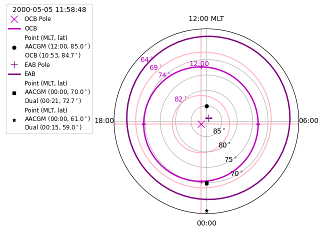
Convert between AACGM and dual-boundary coordinates

Now let us perform the same visualisation using a paired EAB and OCB. The prior example ensured that this was a time with a good dual-boundary for dual from the prior examples. Continue by adding the EAB to the existing figure.

dual.rec_ind = 0
ax.plot(np.radians(dual.eab.phi_cent[dual.eab.rec_ind]),
                   dual.eab.r_cent[dual.eab.rec_ind],
                   "+", color='purple', ms=10, label="EAB Pole")

Calculate and plot the location of the EAB in AACGM coordinates, expanding the radial boundaries of the figure as needed.

dual.get_aacgm_boundary_lats(mlt, rec_ind=dual.rec_ind, overwrite=True)
rad = 90.0 - dual.eab.aacgm_boundary_lat[dual.eab.rec_ind]
ax.plot(theta, rad, "-", color='purple', linewidth=2, label="EAB")
ax.text(theta[40], rad[40] + 2,
        "{:.0f}$^\circ$".format(dual.eab.boundary_lat), fontsize="medium",
        color="m")
ax.set_rmax(np.ceil(max(rad) / 10.0) * 10.0)

Add more reference labels for the dual-boundary coordinates. This is harder to do, because there is no direct conversion beween the dual-boundary coordinates and AACGM coordinates without already knowing the AACGM MLT. To allow forward and backward transformations, normal_coord() also returns the OCB coordinates, which can be reverted using revert_coord(). Without this knowledge, you must provide the AACGM MLT. This is only a barrier for locations equatorward of the OCB.

# Define a latitude grid midway between the EAB and OCB. Since no locations
# at or poleward of the OCB are provided, the reversion will only use the
# shape of the `mlt` arg input.
grid_eab = 0.5 * (dual.ocb.boundary_lat
                  - dual.eab.boundary_lat) + dual.eab.boundary_lat
grid_lat, grid_mlt = dual.revert_coord(grid_eab, mlt, aacgm_mlt=mlt,
                                       is_ocb=False)
grid_lat = 90.0 - grid_lat
grid_theta = grid_mlt * np.pi / 12.0

ax.plot(grid_theta, grid_lat, "-", color="lightpink", zorder=1)
ax.text(grid_theta[40], grid_lat[40] + 2, "{:.0f}$^\circ$".format(grid_eab),
        fontsize="medium", color="m")

# Extend the MLT grid in dual-boundary coordinates
fine_mlt = np.linspace(0, 24.0, num=500)
dual.get_aacgm_boundary_lats(fine_mlt, rec_ind=dual.rec_ind, overwrite=True)
for i, ocb_mlt in enumerate(np.arange(0.0, 24.0, 6.0)):
    ocb_lat, omlt, _ = dual.ocb.normal_coord(
        dual.eab.aacgm_boundary_lat[dual.eab.rec_ind] - 10.0, fine_mlt)
    j = abs(omlt - ocb_mlt).argmin()
    if ocb_mlt == 0:
        j2 = abs(omlt - 24).argmin()
        if abs(omlt[j2] - ocb_mlt) < abs(omlt[j] - ocb_mlt):
            j = j2

    aa, oo = dual.revert_coord(ocb_lat[j], ocb_mlt)
    lon_outer = oo * np.pi / 12.0
    lat_outer = 90.0 - aa

    ax.plot([lon_clock[i], lon_outer], [lat_clock[i], lat_outer], "-",
            color="lightpink", zorder=1)

Now add the location of two more points in AACGM coordinates, calculating the dual-boundary location, and output both coordinates in the legend

aacgm_lat = [70.0, 61.0]
aacgm_mlt = 0.0
bound_lat, bound_mlt, _, _ = dual.normal_coord(aacgm_lat, aacgm_mlt)

markers = ['s', '*']
for i, lat in enumerate(aacgm_lat):
    plabel = "\n".join(["Point (MLT, lat)",
                        "AACGM (00:00, {:.1f}$^\circ$)".format(lat),
                        "Dual ({:02.0f}:{:02.0f}, {:.1f}$^\circ$)".format(
                            np.floor(bound_mlt[i]),
                            (bound_mlt[i] - np.floor(bound_mlt[i])) * 60.0,
                            bound_lat[i])])
    fmt = 'k{:s}'.format(markers[i])
    ax.plot([aacgm_mlt * np.pi / 12.0], [90.0 - lat], fmt, ms=5,
            label=plabel)

Update the legend to finish the figure.

fig.subplots_adjust(left=.3, right=.99)
ax.legend(loc=2, fontsize="small", title="{:}".format(
    dual.dtime[dual.rec_ind]), bbox_to_anchor=(-0.6, 1.15))