Convert between AACGM and OCB coordinates

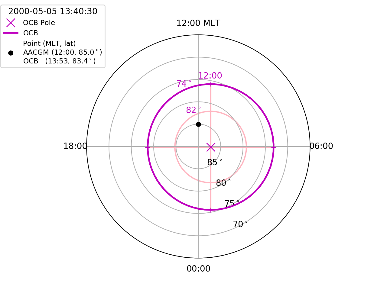
We’ll start by visualising the location of the OCB using the first good OCB in the default IMAGE FUV file.

fig = plt.figure()
ax = fig.add_subplot(111, projection="polar")
ax.set_theta_zero_location("S")
ax.xaxis.set_ticks([0, 0.5*np.pi, np.pi, 1.5*np.pi])
ax.xaxis.set_ticklabels(["00:00", "06:00", "12:00 MLT", "18:00"])
ax.set_rlim(0,25)
ax.set_rticks([5,10,15,20])
ax.yaxis.set_ticklabels(["85$^\circ$", "80$^\circ$", "75$^\circ$",
                         "70$^\circ$"]

Mark the location of the circle centre in AACGM coordinates

ocb.rec_ind = 27
ax.plot(np.radians(ocb.phi_cent[ocb.rec_ind]), ocb.r_cent[ocb.rec_ind],
        "mx", ms=10, label="OCB Pole")

Calculate at plot the location of the OCB in AACGM coordinates

mlt = np.linspace(0.0, 24.0, num=64)
ocb.get_aacgm_boundary_lat(mlt, rec_ind=ocb.rec_ind)
theta = ocbpy.ocb_time.hr2rad(mlt)
rad = 90.0-ocb.aacgm_boundary_lat[ocb.rec_ind]
ax.plot(theta, rad, "m-", linewidth=2, label="OCB")
ax.text(theta[35], rad[35] + 1.5, "74$^\circ$", fontsize="medium", color="m")

Add more reference labels for OCB coordinates. Since we know the location that we want to place these labels in OCB coordinates, the revert_coord() method can be used to get the location in AACGM coordinates.

lon_clock = list()
lat_clock = list()

for ocb_mlt in np.arange(0.0, 24.0, 6.0):
    aa,oo = ocb.revert_coord(74.0, ocb_mlt)
    lon_clock.append(oo * np.pi / 12.0)
    lat_clock.append(90.0 - aa)

ax.plot(lon_clock, lat_clock, "m+")
ax.plot([lon_clock[0], lon_clock[2]], [lat_clock[0], lat_clock[2]], "-",
        color="lightpink", zorder=1)
ax.plot([lon_clock[1], lon_clock[3]], [lat_clock[1], lat_clock[3]], "-",
        color="lightpink", zorder=1)
ax.text(lon_clock[2] + .2, lat_clock[2] + 1.0, "12:00",fontsize="medium",
        color="m")
ax.text(lon[35], olat[35] + 1.5, "82$^\circ$", fontsize="medium", color="m")

Now add the location of a point in AACGM coordinates, calculate the location relative to the OCB, and output both coordinates in the legend

aacgm_lat = 85.0
aacgm_lon = np.pi
ocb_lat, ocb_mlt = ocb.normal_coord(aacgm_lat, aacgm_lon * 12.0 / np.pi)

plabel = "\n".join(["Point (MLT, lat)", "AACGM (12:00, 85.0$^\circ$)",
                    "OCB ({:.0f}:{:.0f},{:.1f}$^\circ$)".format(
                        np.floor(ocb_mlt),
                        (ocb_mlt - np.floor(ocb_mlt)) * 60.0, ocb_lat)])
ax.plot([aacgm_lon], [90.0-aacgm_lat], "ko", ms=5, label=plabel)

Find the location relative to the current OCB. Note that the AACGM coordinates must be in degrees latitude and hours of magnetic local time (MLT).

ocb_lat, ocb_mlt = ocb.normal_coord(aacgm_lat, aacgm_lon * 12.0 / np.pi)
ax.plot([ocb_mlt * np.pi / 12.0], [90.0 - ocb_lat], "mo", label="OCB Point")

Add a legend to finish the figure.

ax.legend(loc=2, fontsize="small", title="{:}".format(
    ocb.dtime[ocb.rec_ind]), bbox_to_anchor=(-0.4, 1.15))

Scaling of values dependent on the electric potential can be found in the ocbpy.ocb_scaling module.